This document is the final report for a project involving an implementation of Lien and Amato’s Approximate Convex Decomposition (ACD) of Polyhedra [1]. The project and initial implementation was started as the final project for 3D Photography in the fall of 2007 and development continued during the spring of 2008.

Intended Applications

Implementing ACD was suggested as a possible project as it can be applied to numerous ongoing research projects at Columbia. The ability to decompose highly complex 3D meshes into a set of convex objects has many immediate applications, including collision detection, rendering, and object recognition.

Of particular importance, are its possible applications to collision detection and object decomposition in grasp planning of robotic actuators, and in consistent decompositions of similarly shaped objects for 3D object recognition and searching.

Approximate Convex Decomposition of Polyhedra

Overview

At its highest level, Approximate Convex Decomposition of Polyhedra can be summarized as follows: given a connected graph of 3D points forming a mesh, iteratively decompose the mesh into a set of submeshes that are at least “approximately” convex. Each mesh is split into two smaller meshes using the plane that best approximates a boundary of high concavity and curvature. Thus, the problem of ACD is primarily that of efficiently estimating the best boundary of high concavity and curvature along which to split the mesh.

Abstraction of Underlying Algorithms

The set of algorithms involved in ACD can all be seen as consisting of the same general pattern, applied at every level: given an existing set of “features” of the polyhedral mesh, compute another derived set of features that are smaller in number yet still approximate the geometry of the object. Next, using both the features of the current level and the new features derived, compute another descriptor relating the features of the derived set.

The description of the algorithm below follows the same format as in the original paper, separating the decomposition into two main sets of algorithms, identifying concave features, and then creating global cuts.

Concave Features

Input Mesh:

The decomposition process begins with the initial input. The first type of “feature” processed is a mesh, consisting of a set of 3D vertices connected by edges in a non-directed graph.

Convex Hull

Using the input mesh, the first stage step is to compute the convex hull of the vertices of the inputted mesh.

Bridges

The next step is to compute “Bridges,” edges that are on the convex hull, but not on the input mesh. Bridges, as the name implies, bridge together vertices of the input mesh that were not originally corrected.

Bridge Groups

Bridges are then combined into “bridge groups,” sets of facets on the convex hull that contain nearly coplanar bridges. In the ACD implementation, only coplanar bridges are combined, while the computational reduction is achieved by using mesh decimation beforehand, rather than in combining roughly coplanar bridges.

Pockets

From bridges groups, one can then compute “pockets.” A pocket is the shortest set of edges (and associated vertices) on the input mesh that connect together two vertices of each bridge group. Note by definition, the vertices and edges of the pocket should consist entirely of vertices and edges that are not on the convex hull.

As explained in the original paper1, pockets can be considered the projection of the convex hull’s bridge edges onto the original mesh.

Global Cuts

Using all of the features identified in the previous section, it is now time to begin the process of splitting the mesh. First, a few more features are required.

Knots

Knots are a subset of the pocket vertices that are deemed most important, referred to as “critical points,” which are defined as the vertices of the pocket that are farthest from the bridge. In the original work, knots are to be calculated by reparametrizing the pocket into “concavity space,” whereby for each vertex in the pocket, the function returns the distance between the vertex and the convex hull, as measured by the distance between the vertex and the bridge.

Pocket Cuts

Using pockets and their associated knots, one next connects knots of adjacent pockets together into pocket cuts, which are sets of connected edges. There are many possible pocket cuts, however one chooses the connections such that each knot only connects to one other knot in an adjacent pocket, simplifying the number of cuts.

Pocket Cut Weights

ACD1 defines the weight of a cut to be:

and γ(κ) = the “accumulated curvature of the edges in κ.”1

Graph Cycles

The set of vertices and edges amongst the pocket cuts form a weighted graph, with the weights of each edge in the cut given in the previous section. The next step is to compute cycles within this graph.

The algorithm starts by first choosing the pocket cut and associated knot with the greatest concavity (by definition, the knot/vertex farthest from the convex hull). Next the minimum spanning tree from the root vertex is calculated, except that after each iteration of the MST algorithm, new vertices are added to the graph, specifically the shortest paths connecting the current paths (via knots) on the input mesh.

More intuitively, the MST is first using strictly the knots to branch out in search of the minimum path. After each iteration of finding the minimum spanning tree, however, it must account for the actual path taken along the input mesh which connects the selected vertices.

Cut Planes

The final step is to use the extracted cycle from the MST to compute a cut plane. ACD defines the plane of best fit for the cycle as the plane minimizing:

where e are the edges of the MST, E the plane of best fit, and μ_E(e) the area between e and the projection of it onto E.

Lastly, the cut plane is used to bisect the model in two.

Implementation

The project consisted of two main phases, initial research and logistical development, and lastly algorithmic implementation development.

Initial Research

The first phase of the project consisted of researching the necessary tools and libraries that would be required to best implement the algorithm, with a long term view that it may be integrated into other projects.

Algorithmic Libraries

CGAL

Two main types of software libraries were required: algorithmic and visual libraries. CGAL[2] (Computational Geometry Algorithms Library) was selected as the primary library upon which to build the entire implementation. In addition, CGAL recently had added integration with the Boost Graph Libraries (BGL).

Boost

Boost[3] is a popular open source set of C++ libraries implementing a vast set of useful algorithms and functionality which provide efficient and portable implementations of several required graph algorithms, including Dijkstras and Minimum Spanning Tree.

Visualization Libraries

Based on past experience, it was deemed essential to create a method of easily visualizing the various stages of algorithms for both debugging and presentation of output. Note that CGAL provides built in support for a number of visualization frameworks. Unfortunately for Windows, it only provides 2D support of its native types.

Therefore several other display libraries and frameworks were investigated, which were used to create two separate methods of displaying the ACD algorithms’ results: the first for debugging and desktop development, the second method for web-based displaying of results (for the project/final report page).

OpenGL

In order to make the software as cross-platform as possible, OpenGL was chosen as the 3D rendering API. More specifically, GLUT[4], or OpenGL Utility Toolkit, was chosen. GLUT is a cross-platform wrapper for OpenGL.

GltZPR

In order to speed development, an additional library built upon GLUT, GltZPR[5] (GLUT Zoom, Pan, Rotate) was also used. GltZPR is a simple library based on GLUT that provides the familiar 3D interface mapping the 3 mouse buttons to zoom, panning, and tilting, respectively, to manipulate the view of the 3D dataset.

GltZPR was used to construct a simple 3D geometry viewer for displaying 1) CGAL’s 3D polyhedron, 2) bridges, and 3) pockets. Its development proceeded instep with the project’s progress and helped enormously in debugging.

JavaView

While searching for open source third-party 3D visualization tools that could directly use CGAL datatypes, I came across Javaview[6]. Javaview, as the name implies, is a free 3D geometry viewer that accepts a number of file formats, and can be embedded within webpages as a java applet.

In addition, I also found a small library, Javaview for CGAL[7], for writing CGAL’s Polyhedron_3 datatype to JavaView’s native file format (JVX). The small library was extended in order to support the custom requirements of ACD, specifically the ability to render both bridges and pockets. Note that all interactive objects displayed within this final report were created using JavaView, Javaview for CGAL, and the additional custom functionality.

Implementation

The description of the implementation is formatted chronologically, in order to best illustrate how the project implementation proceeded and why it developed in manner it did.

Generate Simple Test Case

The first step in implementing the algorithm was to manually develop an initial test input polyhedron similar to one presented in ACD, as shown in Figure 1.

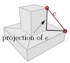
Figure 1 Illustrative Example object Taken from Original Paper, upon which first test object was based.

Limitations of CGAL’s 3D Polyhedral Data Structure

The initial test input was manually created by entering points into CGAL’s default (only) supported Polyhedron_3 input format, OFF. It was at this stage that the first set of problems with using CGAL began to emerge. It turns out that Polyhedron_3, the data structure used by CGAL to store 3D polyhedron’s consisting of vertices, edges, and facets, is extremely limited in the types of meshes it accepts. To this day, the exact requirements or correct complete restricting subset of 3D meshes it not known, but the CGAL documentation states “[CGAL’s implementation] restricts the class of representable surfaces to orientable 2-manifolds – with and without boundary.”[8]

CGAL’s Polyhedron_3 uses an underlying “Half-Edge” data structure, whereby for every edge that is shared by two adjacent facets on the polyhedral surface, two “half-edges” are separately represented, one for each facet. Most importantly, the edges must have opposite directions when defined in the input.

Consider the partial set of edges for the simple cube displayed in Figure 2. Note that the cube is defined as 6 square facets, each defined by 4 edges and 4 vertices. When entering facets into CGAL, either directly or via the OFF file format, note that the order of vertices of each facet is highly important, as it defines the orientation of the edges. CGAL requires that if the frontal facet is defined by (1,2,4,3), then in order for the half-edge connecting the vertices (2,4) to be correct, the right-facing facet must be defined such that 2 comes after four (allowing for wrap-around), for example (4,2,5,6). This becomes significantly more complicated when creating meshes manually that have more than two facets.

This limitation of CGAL’s Polyhedron_3 data structure quickly became the single greatest impediment to implementing the algorithm.

Figure 2 Example Cube with Edge (between vertices 2 and 4) shared by two Facets

Once the edge orientations across all facets were correct, I was able to successfully load the model into CGAL’s data structures, displayed in Figure 3.

Figure 3 First Test Input Polyhedron Utilized During Development

Calculate Convex Hull

One of the reasons for choosing CGAL was because it contained many implementations of required algorithms, including many Convex Hull finding algorithms, supporting several variations for 2D, 3D, and dD convex hulls and Delaunay Triangulations.[9] Specifically, for 3D point sets, it contains 3 primary implementations for convex hull construction:

Static: in which the entire point set is known beforehand and will not change.
Incremental: in which the convex hull can continuously be updated as new points are added.
Dynamic: in which the convex hull is continuously updated as points are both added and removed.

For the implementing of ACD, only the static version is used, as it is the fastest. All methods are mentioned, however, because they may be useful in splitting meshes. Specifically in ACD, after a mesh is split in two, the algorithm then runs again on each submesh, starting by recalculating the convex hull of each submesh. It is conceivable that a faster method may be to leverage the dynamic hull construction algorithm to first duplicate the convex hull of the current mesh so that one has two copies, and then remove the corresponding set of points from each, corresponding to the respective side of the split plane each convex hull represents. This way, rather than completely recalculating the convex hull on complex objects, one can instead copy and then adjust the convex hulls to account for the points removed from the decomposition.

Furthermore, note that there are significant differences in performance between Debug and Release builds, presumably because debug checking is disabled. As such, it is highly recommended to use the Release-compiled code when using for real applications.

The resulting convex hull of the test object is displayed in Figure 4.

Figure 4 Displays the resulting convex hull for the initial test object.

Bridge Calculation

Once the convex hull was calculated, it was then possible to iterate over all its edges, and verify whether the edges were also present on the input mesh, in order to locate bridges.

I initially intended to skip the more advanced part of ACD, whereby bridges are combined in bridge groups, since it only seemed to represent a performance enhancement for complex meshes. I soon discovered at least one very simple case which may have also led the author to introduce the bridge grouping in the first place.

The problem is that the convex hull algorithm returns a polyhedral mesh (including facets) that does not take into account the facets of the existing mesh. Specifically, if facets on the input mesh consisted of more than three vertices, then the convex hull will likely return a convex hull polyhedral mesh which arbitrarily splits the facet into smaller 3-vertex facets. Then, if one attempts to locate bridges (edges that are not on the input mesh but that are on the convex hull), one will also select edges that while still on the surface of the input mesh, were not explicitly defined as edges of the input mesh. The result is that false bridges that bisect input mesh facets are found, as displayed in Figure 5a.

Figure 5 (a) False Bridges resulting from Input Meshes with facets containing more than three vertices. (b) Resulting bridges after coplanar facets are removed from convex hull.

Therefore, it became necessary to in fact implement at least a simple form of bridge group. The method chosen was for each bridge, to iterate over all of its facets, and if any were coplanar, to remove the bridge. The result was that bridges that came from edges that were explicitly defined in the original input mesh, but were completely on the surface of the input mesh, were removed. The filtered set of bridges is displayed in Figure 5b.

Calculate Pockets

With the correct bridges located, it was now time to implement pocket calculation.

For each bridge, one calculates the corresponding pocket by using Dijkstra’s algorithm on the input mesh, and locating the shortest distance on the mesh connecting the two vertices of the bridge.

One of the primary reasons for choosing CGAL was because not only did it provide the necessary geometric algorithms, but it also had bindings that allowed the use of the Boost Graph Libraries, which included an implementation of Dijkstra’s, directly on CGAL’s data structures.

After weeks of struggling to get CGAL’s BGL bindings to successfully compile and run without crashing, the true culprit was found.

Bugs in CGAL’s BGL Bindings

After exhaustively searching the CGAL mailing list, an email was discovered, dated 2007-11-17, that precisely described the exact same compilation problem I had been having. It turned out that there was a bug in CGAL’s BGL code that instructed BGL how to access CGAL’s Polyhedron_3 as a generic BGL graph. After emailing the CGAL developer and obtaining a copy of the corrected source code, I was finally able to compile my program and run Dijkstra’s.

More Bugs in CGAL

At this stage, I was now able to run Dijkstra’s algorithm, providing as input the polyhedral mesh and target pair of vertices for the bridge. Unfortunately, the results were wrong.

Additional searching of the mailing list did not provide any additional results.

After exhaustive debugging, I was eventually able to trace the problem again to CGAL. A common time-saving programming practice is to compare the squared distances of points, as opposed to actually computing the distances, requiring the calculation of two square roots. Unfortunately, this optimization does not hold once one is taking the summation of several distances. The bug was caused by CGAL reporting the weight of each edge in the mesh as the squared distance of the vertices, instead of the distance. After fixing the code, Dijkstra’s finally seemed to work correctly, and I was able to successfully calculate pockets (shown below).

Using More Complex Objects

While searching the mailing list for solutions to the previously discussed bugs, I also came across a number of other emails describing possible bugs and problems others had when using the convex hull routines on large input meshes. This motivated me to first try loading one of the complex meshes presented in ACD, before moving on to the second portion of the algorithm. I settled on the Stanford bunny.

Object File Formats

CGAL provides support for writing out many formats, but oddly only contains an input reader for only one file format: OFF. After finding out first hand the difficulty of manually inputting a mesh into CGAL’s Polyhedron_3 class, I am curious if it is a direct result of the extremely limited class of objects.

Unfortunately, I could not find OFF-formatted versions of the Stanford bunny, and realizing that the intended application of the implementation was to accept arbitrary meshes that were most likely not going to be in OFF format, it was necessary to find a method of converting other formats into OFF.

In addition to the official API, CGAL comes with numerous examples (located in *CGAL installation directory*\examples\Polyhedron_IO) converting OFF files to other common formats (iv, stl, vrml, and wav). It also contains a single utility for converting Inventor files (IV) into OFF. Note that the Stanford bunny[10] is stored in Stanford’s PLY format. On their main page, they also make available a tool for converting their PLY format to IV. After downloading and compiling all of the tools, I consecutively ran each tool, until finally reaching an OFF-formatted bunny.

Duplicate Points

Upon loading the Stanford bunny and running the algorithm, the results were clearly wrong. After several sessions of debugging, I finally realized that in converting the formats, somewhere along the line, duplicate points had been added to the mesh, perhaps even to satisfy the same persistent Half-edge constraint previously discussed.

Eventually, after trying several third party 3D object format converters, I was finally able to find a combination of different programs capable of sufficiently processing the mesh in order to both remove any duplicate points and generate a file that could be correctly converted into OFF and loaded by CGAL, as shown in Figure 6.

First, the input mesh is loaded with Mesh Editor[11] and was then decimated and resaved. Then the mesh was loaded into 3D Object Converter.[12]

Figure 6 Stanford Bunny Loaded into ACD Implementation. (a) Original Input mesh. (b) Convex Hull of Input Mesh. (c) Bridges (in Blue) and Pockets (in Green) on the bunny.

Conclusions

Implementation Status

At this stage of development, the single greatest hurdle is the still the limitations in CGAL’s Polyhedron_3 data structure. The biggest road block is that once a cut plane is found, it is not clear how to split the mesh into two, without breaking the mesh restrictions. While still searching for the solution and monitoring CGAL’s mailing list, I have also begun to look for other mesh and computational geometry libraries to use in place of CGAL.

It is somewhat re-assuring to know that I am not the only one having difficulty implementing the algorithm. On Lien’s ACD project page1, he states that he too is currently working on implementing ACD as well, and that one should check back later for a future release.

Lessons Learned

While I wasn’t able to finish the implementation yet, I still learned a lot in doing this problem. I gained significant exposure to computational geometry, a field I had extremely little knowledge about prior to starting this project.

I also gained experience using OpenGL and variety of 3D visualization programs. I wrote my very first OpenGL program while doing this project in order to visualize the meshes.

Lastly, I learned the importance of strictly adhering to the rule of acknowledging sunken costs and changing direction if needed. If I could do it all over again, I would have abandoned CGAL early on, rather than persisted in using it and struggling with all the problems its use created, especially after realizing that it had several significant bugs.

Appendix

Development Environment

The project was developed utilizing Microsoft Visual Studio’s Visual C++ Express 2005, available free for download. In addition it requires the installation of both CGAL and Boost.

Submitted Materials

Directories contained within project archive:

ADC_Solution:

contains the MSVC++ Solution, project, and all source code.

CGAL_Bugfixes:

Contains the modified files that fix the CGAL bugs, includes both the fixes sent from Andreas Fabri, and the fix I added to correct the Distance bug.

Executable:

Contains a “Release” build of the actual program. Execute with “ACD.exe latest_bunny.off” for example.

References

Table of Contents